

Contents
- What does Granger causality mean?
- The test in two regressions
- Step-by-step procedure
- Step 1: Check stationarity
- Step 2: Select the lag length
- Step 3: Run the test in both directions
- Step 4: Read and report the result
- Worked example: wholesale and retail shallot prices
- What earlier real-data analysis showed
- Running the test in EViews, R, and Python
- Common mistakes
- Frequently asked questions
- Does Granger causality prove cause and effect?
- Which lag length should be used in a Granger causality test?
- What if the data are not stationary?
- Can Granger causality run in both directions?
- What is the difference between Granger causality and cointegration?
- References and further reading
Versi bahasa Indonesia: Uji Kausalitas Granger
Short answer: The Granger causality test checks whether the past values of one time series improve the prediction of another series beyond what that series’ own past already explains. If they do, the first series “Granger-causes” the second. The test compares two regressions with an F-test, after the series have been made stationary and the lag length has been selected with an information criterion. It identifies predictive precedence, not true cause and effect.
What does Granger causality mean?
Clive Granger (1969) proposed a simple and testable definition of causality for time series: a variable X causes a variable Y if past values of X contain information that helps predict Y, over and above the information contained in past values of Y. The idea became a standard tool of applied econometrics, and Granger later received the 2003 Nobel Memorial Prize in Economic Sciences, shared with Robert Engle, for his work on time series methods.
The word “causality” is the source of most misinterpretations. A significant result shows that X moves first and that its movements carry predictive information about Y; however, both series may simply respond, at different speeds, to a third factor that is not in the model. Thus, the result is best reported as “X Granger-causes Y” rather than “X causes Y”.
The interactive chart below uses the simulated data of the worked example. Moving the slider shifts the wholesale price forward in time; at a lag of two months, its movements line up with the later movements of the retail price.
Wholesale price Retail price
Move the slider to shift the wholesale price.
The test in two regressions
For a lag length p, the test estimates two models. The restricted model explains Y with its own past only: Yt = a0 + a1Yt−1 + … + apYt−p + et. The unrestricted model adds the past of X: … + b1Xt−1 + … + bpXt−p. The null hypothesis states that all b coefficients are zero, meaning that X does not Granger-cause Y. An F-test compares the residual sums of squares of the two models; a p-value below 0.05 rejects the null hypothesis. The test is then repeated in the opposite direction, because the relationship can be unidirectional, bidirectional, or absent.
Step-by-step procedure
Step 1: Check stationarity
The F-test assumes stationary series. Prices, production, and most macroeconomic variables in levels are not stationary; consequently, a test on levels can produce spurious significance. The Augmented Dickey–Fuller (ADF) test is applied to each series in levels and in first differences. A series that is non-stationary in levels but stationary in first differences is integrated of order one, I(1), and the test is run on the differenced data. When the series are cointegrated and the long-run information in levels matters, the Toda and Yamamoto (1995) procedure is a well-established alternative.
Step 2: Select the lag length
The result depends strongly on the lag length. Instead of choosing a lag arbitrarily, the lag is selected with information criteria from a vector autoregression (VAR) of the two series: the Akaike (AIC), Schwarz (SC), and Hannan–Quinn (HQ) criteria. The lag with the lowest value is preferred. When the criteria disagree, SC usually selects a shorter model and AIC a longer one; both choices can be reported as a robustness check.
Step 3: Run the test in both directions
The test is run for X → Y and for Y → X using the selected lag. Most software reports both directions in one table.
Step 4: Read and report the result
Each direction produces an F-statistic, its degrees of freedom, and a p-value. A complete report states the transformation of the data, the lag length and how it was chosen, and the F-statistic with its p-value for each direction, for example “wholesale prices Granger-cause retail prices (F(2, 64) = 45.31; p < 0.001), whereas the reverse is not significant (F(2, 64) = 1.19; p = 0.31)”.
Worked example: wholesale and retail shallot prices
The example uses 72 months (2019–2024) of simulated wholesale and retail shallot prices in rupiah per kilogram, constructed so that retail prices react to wholesale prices with a delay of about two months. The data are labeled as simulated and can be downloaded for practice: granger-example-shallot-prices.csv.
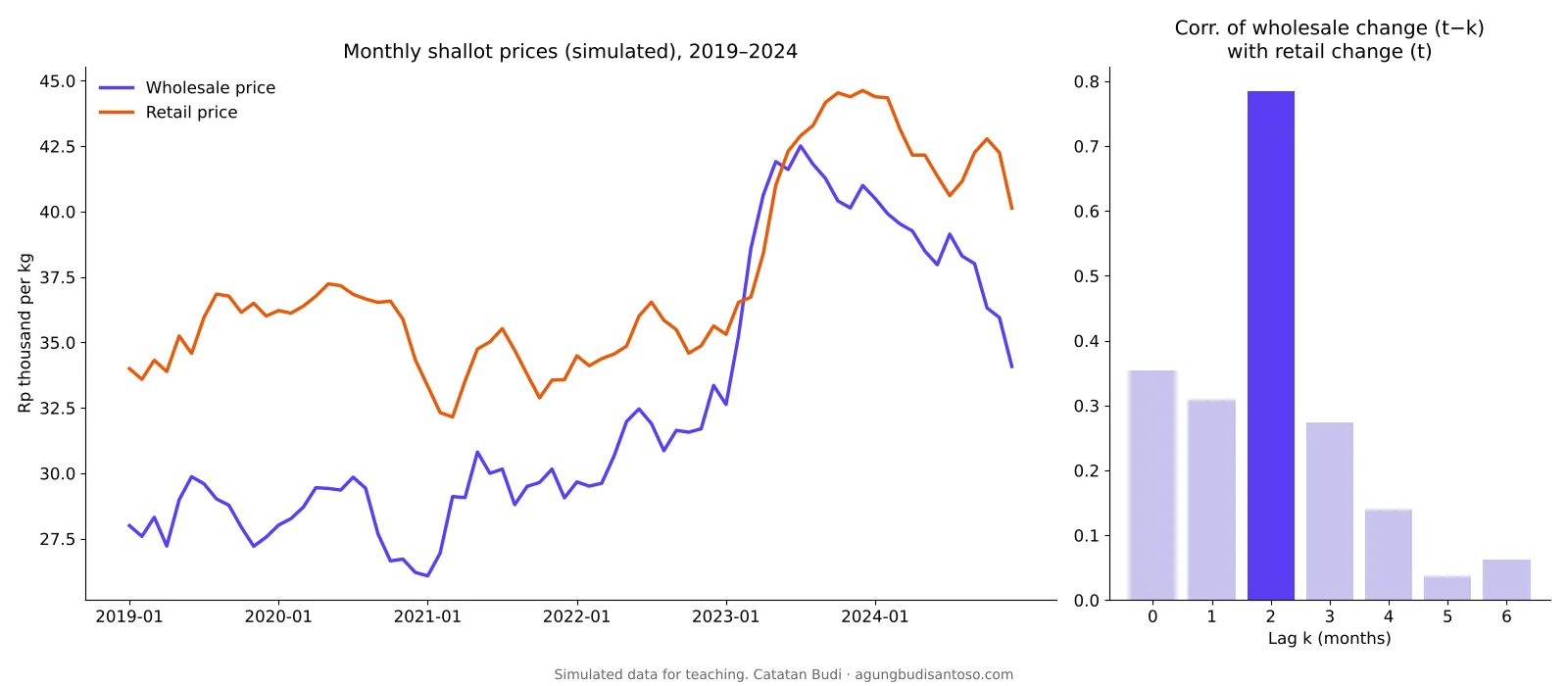
The ADF test (with a constant) does not reject a unit root in levels, yet rejects it clearly in first differences (Table 1). Both series are therefore I(1), and the test is applied to monthly price changes.
| Series | ADF statistic, levels | ADF statistic, first differences | Conclusion |
|---|---|---|---|
| Wholesale price | −1.31 | −3.72 | I(1) |
| Retail price | −1.68 | −3.70 | I(1) |
Table 1. The 5% critical value for this sample size is about −2.90.
All three information criteria select a lag of two months (Table 2), which matches the delay built into the data.
| Lag | AIC | SC | HQ |
|---|---|---|---|
| 1 | 26.755 | 26.889 | 26.808 |
| 2 | 26.145 | 26.413 | 26.251 |
| 3 | 26.252 | 26.654 | 26.411 |
| 4 | 26.336 | 26.871 | 26.547 |
Table 2. VAR lag selection on first differences (maximum lag 6; lags 5 and 6 omitted, both higher).
The Granger test results show a clear unidirectional relationship (Table 3). At the selected lag, wholesale price changes Granger-cause retail price changes (F(2, 64) = 45.31; p < 0.001), whereas retail price changes do not Granger-cause wholesale price changes (F(2, 64) = 1.19; p = 0.31). With a lag of one month, the relationship is only marginal (p = 0.068); this underscores why the lag must be selected with a criterion rather than by habit.
| Lag | Wholesale → Retail: F | p-value | Retail → Wholesale: F | p-value |
|---|---|---|---|---|
| 1 | 3.43 | 0.068 | 0.96 | 0.330 |
| 2 | 45.31 | < 0.001 | 1.19 | 0.311 |
| 3 | 26.67 | < 0.001 | 0.66 | 0.582 |
| 4 | 20.49 | < 0.001 | 1.14 | 0.348 |
Table 3. Granger causality tests on first differences of simulated data.
In market terms, price signals in this simulated system travel downstream from wholesalers to retailers with a delay of about two months, and not in the opposite direction. Thus, monitoring wholesale prices would provide an early warning of retail price movements.
What earlier real-data analysis showed
An earlier analysis on Catatan Budi applied the same test to monthly rice prices in North Sumatra from 2016 to 2019 (48 observations, Ministry of Agriculture data). The vertical chain, from the farm-gate price of dry grain to the miller price and the consumer price of rice, showed no Granger causality at a lag of two months. Conversely, the horizontal relationship between two markets in Medan, Aksara and Petisah, was significant: prices at Aksara Granger-caused prices at Petisah. The contrast suggests that price transmission between neighboring retail markets was faster than transmission along the marketing chain. A re-analysis of such data should begin with the stationarity check and lag selection described above.
Running the test in EViews, R, and Python
In EViews, the series are opened as a group, and the test is available under Quick → Group Statistics → Granger Causality Test, where the lag length is entered. The output lists both directions with F-statistics and probabilities.
In R, the lmtest package provides grangertest(retail ~ wholesale, order = 2, data = d), which tests whether wholesale Granger-causes retail. The vars package offers VARselect() for lag selection.
In Python, the statsmodels library provides the test. The column order matters: the function tests whether the second column Granger-causes the first.
import pandas as pd
from statsmodels.tsa.stattools import adfuller, grangercausalitytests

df = pd.read_csv("granger-example-shallot-prices.csv")
d = df[["retail", "wholesale"]].diff().dropna()    # first differences

print(adfuller(df["retail"])[0], adfuller(d["retail"])[0])
res = grangercausalitytests(d, maxlag=2)            # H0: wholesale does not Granger-cause retail
Common mistakes
Five mistakes appear repeatedly in theses and manuscripts: (1) running the test on non-stationary levels without a cointegration-aware procedure; (2) choosing the lag arbitrarily, often lag 1 or lag 2, without an information criterion; (3) testing only one direction; (4) interpreting a significant result as proof of cause and effect; and (5) omitting the lag length, the data transformation, or the degrees of freedom from the report. Each of these mistakes changes either the result or the reader’s ability to verify it.
Frequently asked questions
Does Granger causality prove cause and effect?
No. Granger causality shows that one series helps predict another, which implies temporal precedence. A common driver outside the model, expectations, or omitted variables can produce the same pattern. The result supports, but does not establish, a causal interpretation; theory and institutional knowledge are still required.
Which lag length should be used in a Granger causality test?
The lag should be selected with information criteria (AIC, SC, or HQ) from a VAR of the series. Monthly data commonly require longer lags than annual data. Reporting the result for neighboring lags is a useful robustness check, as Table 3 illustrates.
What if the data are not stationary?
Non-stationary series are usually differenced until they become stationary, and the test is run on the differences. When the series are cointegrated, a vector error correction model or the Toda–Yamamoto procedure preserves the long-run information that differencing removes.
Can Granger causality run in both directions?
Yes. When X Granger-causes Y and Y Granger-causes X, the relationship is bidirectional, which often indicates feedback, for example between prices in two connected markets.
What is the difference between Granger causality and cointegration?
Cointegration concerns a stable long-run relationship between non-stationary series, whereas Granger causality concerns short-run predictive precedence. If two series are cointegrated, Granger causality must exist in at least one direction, which is why the two analyses are often reported together.
References and further reading
- Granger, C. W. J. (1969). Investigating causal relations by econometric models and cross-spectral methods. Econometrica, 37(3), 424–438.
- Toda, H. Y., & Yamamoto, T. (1995). Statistical inference in vector autoregressions with possibly integrated processes. Journal of Econometrics, 66(1–2), 225–250.
- Lütkepohl, H. (2005). New Introduction to Multiple Time Series Analysis. Springer.
- Indonesian version with the EViews screenshots: Uji Kausalitas Granger: Pengertian dan Contohnya.
- Stationarity in time series (Indonesian): Uji Stasioneritas Data Time Series.

Discussion
No comments yet. Have a question about this topic? Write it below and I will do my best to answer.